Note

This static document was automatically created from the output of a jupyter notebook.

Execute and modify the notebook online here.

Implementing Beamformers

This Jupyter notebook will outline the step-by-step process of implementing a new receiving beamformer within the HermesPy framework, using the Minimum Variance Distortionless Response (MVDR, also known as [Cap69]) beamformer as a working example.

As an initial step we will import all required modules:

import numpy as np

from hermespy.core import AntennaArray
from hermespy.beamforming import ReceiveBeamformer

The Capon beamformer estimates the power \(\hat{P}\) received from a direction \((\theta, \phi)\), where \(\theta\) is the zenith and \(\phi\) is the azimuth angle of interest in spherical coordinates, respectively. Let \(Y \in \mathbb{C}^{M \times N}\) be the the matrix of \(N\) time-discrete samples acquired by an antenna arrary featuring \(M\) antennas and

\begin{equation} \mathbf{R} = \mathbf{Y}\mathbf{Y}^{\mathsf{H}} \end{equation}

be the respective sample correlation matrix. The antenna array’s response towards a source within its far field emitting a signal of small relative bandwidth is \(\mathbf{a}(\theta, \phi) \in \mathbb{C}^{M}\). Then, the Capon’s spatial power response is defined as

\begin{equation} \hat{P}_{\mathrm{Capon}}(\theta, \phi) = \frac{1}{\mathbf{a}^{\mathsf{H}}(\theta, \phi) \mathbf{R}^{-1} \mathbf{a}(\theta, \phi)} \end{equation}

with

\begin{equation} \mathbf{w}(\theta, \phi) = \frac{\mathbf{R}^{-1} \mathbf{a}(\theta, \phi)}{\mathbf{a}^{\mathsf{H}}(\theta, \phi) \mathbf{R}^{-1} \mathbf{a}(\theta, \phi)} \in \mathbb{C}^{M} \end{equation}

being the beamforming weights to steer the sensor array’s receive characteristics towards direction \((\theta, \phi)\), so that

\begin{equation} \tilde{\mathbf{y}}(\theta, \phi) = \mathbf{w}^\mathsf{H}(\theta, \phi) \mathbf{Y} \end{equation}

are the estimated signal samples impinging onto the sensor array from said direction.

The structure of receiving beamformers is implemented as an abstract prototype in the ReceiveBeamformer. Prototypes specify several abstract properties and methods which inheriting classes must implement. For receiving beamformers those are

• num_receive_input_streams - Number of antenna streams the beamformer can process.Our Capon implementation will always require the samples of all device antennas.

• num_receive_output_streams - Number of antenna streams the beamformer generates after processing.Since the Capon beamformer focuses the power towards a single direction of interest per estimation, a single stream of samples will be generated after beamforming.

• num_receive_focus_angles - Number of angles of interest the beamformer requires for its configuration.The same logic as before applies, only a single direction of interest per beamforming operation is required.

• _decode() - This subroutine performs the actual beamforming, given an array of baseband samples, assumed carrier frequency and the angles of interest. This is where the Capon algorithm is being implemented.

class CaponBeamformer(ReceiveBeamformer):

    def __init__(self, *args, **kwargs) -> None:

        ReceiveBeamformer.__init__(self, *args, **kwargs)

    @property
    def num_receive_input_streams(self) -> int:
        return self.operator.device.num_receive_ports

    @property
    def num_receive_output_streams(self) -> int:
        return 1

    @property
    def num_receive_focus_points(self) -> int:
        return 1

    def _decode(
        self,
        samples: np.ndarray,
        carrier_frequency: float,
        angles: np.ndarray,
        array: AntennaArray,
    ) -> np.ndarray:

        # Compute the inverse sample covariance matrix R
        sample_covariance = np.linalg.inv(samples @ samples.T.conj() + np.eye(samples.shape[0]))

        # Query the sensor array response vectors for the angles of interest and create a dictionary from it
        dictionary = np.empty((array.num_receive_antennas, angles.shape[0]), dtype=complex)
        for d, focus in enumerate(angles):
            array_response = array.spherical_phase_response(carrier_frequency, focus[0, 0], focus[0, 1])
            dictionary[:, d] = sample_covariance @ array_response / (array_response.T.conj() @ sample_covariance @ array_response)

        beamformed_samples = dictionary.T.conj() @ samples
        return beamformed_samples[:, np.newaxis, :]

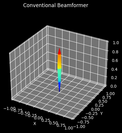
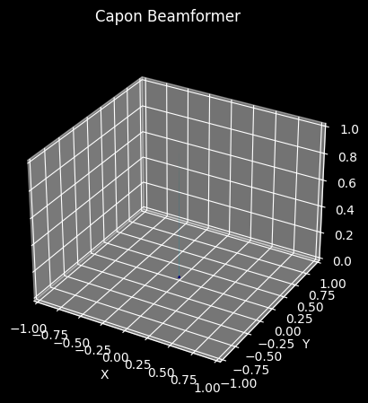
And that’s it, by specifying three properties and the decode routine a new beamformer has been implemented within HermesPy. We can now plot the beamforming characteristics towards a signal impinging from \((\theta = 0, \phi = 0)\) by calling plot_pattern and compare it to the CoventionalBeamformer:

import matplotlib.pyplot as plt

from hermespy.core import AntennaMode
from hermespy.beamforming import ConventionalBeamformer
from hermespy.simulation import SimulatedUniformArray, SimulatedIdealAntenna

# Create a simulated uniform linear array with 8x8 antennas
carrier_frequency = 72e9
half_wavelength = 1.5e8 / carrier_frequency
array = SimulatedUniformArray(SimulatedIdealAntenna, half_wavelength, (8, 8, 1))

# Configure beamformers
conventional = ConventionalBeamformer()
capon = CaponBeamformer()

# Render the beamformer's characteristics
_ = array.plot_pattern(carrier_frequency, conventional, title="Conventional Beamformer")
_ = array.plot_pattern(carrier_frequency, capon, title="Capon Beamformer")
plt.show()

We may now use the newly created beamforming class to configure receive signal processing chains within HermesPy. For example, within an imaging radar application simulation:

import numpy as np
from scipy.constants import pi, speed_of_light

from hermespy.core import dB, ConsoleMode
from hermespy.channel import SingleTargetRadarChannel
from hermespy.simulation import Simulation, SimulatedIdealAntenna, SimulatedUniformArray
from hermespy.radar import Radar, FMCW, ReceiverOperatingCharacteristic

# Create a new simulation featuring a single device transmitting at 10GHz
simulation = Simulation(console_mode=ConsoleMode.SILENT)
device = simulation.scenario.new_device(antennas=SimulatedUniformArray(SimulatedIdealAntenna, .5 * speed_of_light / 10e9, (3, 3)))
device.carrier_frequency = 10e9

radar_channel = SingleTargetRadarChannel(target_range=10., radar_cross_section=1., attenuate=False)
simulation.scenario.set_channel(device, device, radar_channel)

# Configure a radar operation on the device
radar = Radar()
radar.device = device
radar.waveform = FMCW()
radar.receive_beamformer = CaponBeamformer()

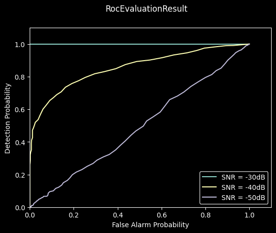
simulation.add_evaluator(ReceiverOperatingCharacteristic(radar, radar_channel))
simulation.new_dimension('snr', dB(-18, -21, -25))
simulation.num_samples = 1000

radar.receive_beamformer.probe_focus_points = np.array([[0., 0.]])
result = simulation.run()

_ = result.plot()
plt.show()

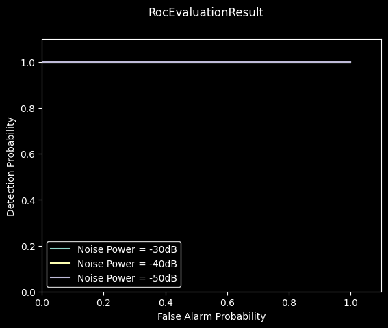
When focusing our beamformer away from the direction of the reflecting target, the target’s echo signal will be attenuated, and therefore the detection probability will decrease:

radar.receive_beamformer.probe_focus_points = np.array([[.5*pi, .5*pi]])
result = simulation.run()

_ = result.plot()
plt.show()