Note

This static document was automatically created from the output of a jupyter notebook.

Execute and modify the notebook online here.

Implementing Evaluators

Evaluators represent the process of estimating performance indicators within Hermes’ API, both during simulation runtime and in custom use-cases. They are, arguably, one of the more complex concepts to grasp for library users not very accustomed to distributed computing.

In order to demonstrate the programming workflow, we’ll add an evaluator estimating the average signal power received at a wireless device. Such an tool could be useful to gain insight into the behaviour of beamformers in multipath environments, or simply as a debugging tool of channel models and waveforms. Let’s get right into it:

from __future__ import annotations
from typing import List

import matplotlib.pyplot as plt
import numpy as np

from hermespy.core import Artifact, Evaluation, EvaluationResult, Evaluator, Executable, GridDimension, Receiver, Signal


class PowerArtifact(Artifact):

    power: float

    def __init__(self, power: float) -> None:

        self.power = power

    def __str__(self) -> str:

        return f"{self.power:.2f}"

    def to_scalar(self) -> float:

        return self.power


class PowerEvaluation(Evaluation):

    power: np.ndarray

    def __init__(self, signal: Signal) -> None:

        self.power = signal.power

    def plot(self) -> None:

        with Executable.style_context():

            fig, axis = plt.subplots()
            fig.suptitle('Received Signal Powers')

            axis.stem(np.arange(len(self.power)), self.power)
            axis.set_xlabel('Antenna Index')
            axis.set_ylabel('Power')

    def artifact(self) -> PowerArtifact:

        summed_power = np.sum(self.power, keepdims=False)
        return PowerArtifact(summed_power)


class PowerEvaluationResult(EvaluationResult):

    def __init__(
        self,
        grid: List[GridDimension],
        evaluator: PowerEstimator,
        artifacts: np.ndarray,
    ) -> None:

        self.mean_powers = np.empty(artifacts.shape, dtype=float)
        for section_coords in np.ndindex(artifacts.shape):
            self.mean_powers[section_coords] = np.mean([a.power for a in artifacts[section_coords]])

        EvaluationResult.__init__(self, grid, evaluator)

    def _plot(self, axes: plt.Axes) -> None:

        self._plot_multidim(self.mean_powers, 0, 'Average Power', 'linear', 'linear', axes)

    def to_array(self) -> np.ndarray:

        return self.mean_powers


class PowerEstimator(Evaluator):

    def __init__(self, receiver: Receiver) -> None:

        self.__receiver = receiver
        Evaluator.__init__(self)

    def evaluate(self) -> PowerEvaluation:

        if self.__receiver.reception is None:
            raise RuntimeError("Receiver has not reception available to evaluate")

        return PowerEvaluation(self.__receiver.reception.signal)

    @property
    def abbreviation(self) -> str:

        return "Power"

    @property
    def title(self) -> str:

        return "Received Power"

    def generate_result(self, grid: List[GridDimension], artifacts: np.ndarray) -> PowerEvaluationResult:

        return PowerEvaluationResult(grid, self, artifacts)

Here’s what you’re probably thinking right now: Artifacts, Evaluations, EvaluationResults and Evaluators, why do we need four interacting classes to investigate a single performance indicator? The answer is, this structure is required to enable efficient distributed execution of Monte Carlo simulations, while simulatenously offering an easily programmable interface for other use-cases such as software defined radio operation.

The basis is the Evaluator, in our case the PowerEstimator. Given a single scenario data drop, it generates an Evaluation object representing the extracted performance indicator information. This information is then compressed to Artifacts Artifacts for each simulation grid sample and finally collected within the generate_result method of the Evaluator, creating an EvaluationResult.

During distributed simulations, the process of generating Artifacts is executed multiple times in parallel, with only the resulting artifacts being sent to the simulation controller, in order to optimize the simulation data throughput between simulation controller and distributed simulation workers. Hermes is built around the Ray, with optimizations like this Monte Carlo simulations become “embarassingly parallel” and, as a consequence, blazingly fast on multicore systems.

We can now define the simulation scenario of a two-device \(5 \times 5\) MIMO simplex link transmitting an OFDM waveform over an ideal channel. Within a Monte Carlo simulation, we sweep the channel gain and observe the effect on the received signal power by our newly created Estimator:

from hermespy.core import ConsoleMode, dB
from hermespy.modem import SimplexLink, ElementType, FrameElement, FrameResource, FrameSymbolSection, OFDMWaveform, SpatialMultiplexing
from hermespy.simulation import Simulation, SimulatedIdealAntenna, SimulatedUniformArray


# Create a new Monte Carlo simulation
simulation = Simulation(console_mode=ConsoleMode.SILENT)

# Configure a simplex link between a transmitting and receiving device, interconnected by an ideal channel
link = SimplexLink(simulation.new_device(antennas=SimulatedUniformArray(SimulatedIdealAntenna, 1e-2, [5, 1, 1])),
                   simulation.new_device(antennas=SimulatedUniformArray(SimulatedIdealAntenna, 1e-2, [5, 1, 1])))

# Configure an OFDM waveform with a frame consisting of a single symbol section
link.waveform = OFDMWaveform(resources=[FrameResource(elements=[FrameElement(ElementType.DATA, 1024)])],
                                       structure=[FrameSymbolSection(pattern=[0])])
link.precoding[0] = SpatialMultiplexing()

# Configure a sweep over the linking channel's gain
simulation.new_dimension('gain', dB(0, 2, 4, 6, 8, 10),
                         simulation.scenario.channel(link.transmitting_device, link.receiving_device),
                         title="Channel Gain")

# Configure our custom power evaluator
power_estimator = PowerEstimator(link)
simulation.add_evaluator(power_estimator)

# Run the simulation
result = simulation.run()

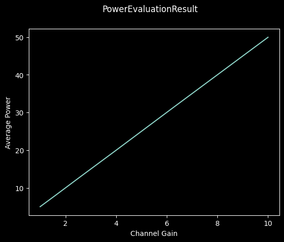
The simulation routine automatically distributes the workload to all detected CPU cores within the system (in this case \(24\)) and generates PowerArtifact objects in parallel. Once the simulation is finished, a single PowerEvaluationResult is generated and stored within a MonteCarloResult returned by the simulation run method.

Calling the result’s plot method will then internally call the evaluation result’s plot, resulting in the following performance indicator visualization:

_ = result.plot()
plt.show()

Now while this renders the average power over a number of samples within a simulation, the Hardware Loop has a feature representing performance indicator information in real time during data collection.

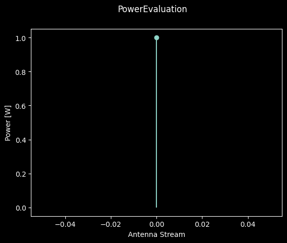
This is internally realized by calling the plot funtion of evaluations generated by evaluators, before they are being compressed to artifacts. We can demonstrate the output in our current simulation scenario by generating a single drop and calling the evaluator:

_ = simulation.scenario.drop()

power_estimator.evaluate().plot()
plt.show()