Selective Leakage¶

The selective leakage implementation allows for the definition of frequency-domain filter characteristics for each transmit-receive antenna pair within a radio-frequency frontend.

Configuring a SimulatedDevice's with a selective isolation model is achived by setting the isolation property of an instance.

# Create a new device
simulation = Simulation()
device = simulation.new_device()

# Specify the device's isolation model with a high-pass characteristic
leakage_frequency_response = np.zeros((1, 1, 101))
leakage_frequency_response[0, 0, :50] = np.linspace(1, 0, 50, endpoint=False)
leakage_frequency_response[0, 0, 50:] = np.linspace(0, 1, 51, endpoint=True)
leakage_impulse_response = ifft(ifftshift(leakage_frequency_response))
device.isolation = SelectiveLeakage(leakage_impulse_response)

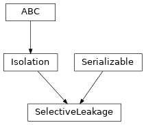
class SelectiveLeakage(leakage_response, *args, **kwargs)[source]¶

Bases: Serializable, Isolation

Model of frequency-selective transmit-receive leakage.

Parameters:: leakage_response (np.ndarray) – Three-dimensional leakge impulse response matrix \(\mathbf{H}\) of dimensions \(M \times N \times L\), where \(M\) is the number of receive streams and \(N\) is the number of transmit streams and \(L\) is the number of samples in the impulse response.
Raises:: ValueError – If the leakage response matrix has invalid dimensions.

classmethod Normal(device, num_samples=100, mean=1.0, variance=1.0)[source]¶

Initialize a frequency-selective leakage model with a normally distributed frequency response.

Parameters:

mean (float, optional) – Mean of the frequency response in real and imaginary parts. One by default.
variance (float, optional) – Variance of the frequency response in real and imaginary parts. One by default.

Return type:

SelectiveLeakage

Returns: An initialized selective frequency model.

property leakage_response: ndarray¶

Leakage impulse response matrix.

Numpy matrix of dimensions \(M \times N \times L\), where \(M\) is the number of receive streams and \(N\) is the number of transmit streams and \(L\) is the number of samples in the impulse response.