Antenna Descriptions

Antenna Configuration

class AAT

Type of antenna array.

alias of TypeVar(‘AAT’, bound=AntennaArray)

class APT

Type of antenna port.

alias of TypeVar(‘APT’, bound=AntennaPort)

class AT

Type of antenna.

alias of TypeVar(‘AT’, bound=Antenna)

class Antenna(mode=AntennaMode.DUPLEX, pose=None)

Bases: ABC, Generic[APT], Transformable, Serializable

Model of a single antenna.

A set of antenna models defines an antenna array model.

Parameters:

• mode (AntennaMode, optional) – Antenna’s mode of operation. By default, a full duplex antenna is assumed.

• pose (Transformation, optional) – The antenna’s position and orientation with respect to its array.

abstract copy()

Create a deep copy of the antenna.

Return type:

TypeVar(AT, bound= Antenna)

Returns:

A deep copy of the antenna.

global_characteristics(global_direction)

Query the antenna’s polarization characteristics towards a certain direction of interest.

Parameters:

global_direction (Direction) – Cartesian direction unit vector of interest.

Return type:

ndarray

Returns:

Two-dimensional numpy vector representing the antenna’s polarization components.

abstract local_characteristics(azimuth, elevation)

Generate a single sample of the antenna’s characteristics.

The polarization is characterized by the angle-dependant field vector

\[\begin{split}\mathbf{F}(\phi, \theta) = \begin{pmatrix} F_{\mathrm{H}}(\phi, \theta) \\ F_{\mathrm{V}}(\phi, \theta) \\ \end{pmatrix}\end{split}\]

denoting the horizontal and vertical field components. The directional antenna gain can be computed from the polarization vector magnitude

\[\begin{split}A(\phi, \theta) &= \lVert \mathbf{F}(\phi, \theta) \rVert \\ &= \sqrt{ F_{\mathrm{H}}(\phi, \theta)^2 + F_{\mathrm{V}}(\phi, \theta)^2 }\end{split}\]

Parameters:

• azimuth (float) – Considered horizontal wave angle in radians \(\phi\).

• elevation (float) – Considered vertical wave angle in radians \(\theta\).

Return type:

ndarray

Returns:

Two dimensional numpy array denoting the horizontal and vertical ploarization components of the antenna response vector.

plot_gain(angle_resolution=180)

Visualize the antenna gain depending on the angles of interest.

Parameters:

angle_resolution (int, optional) – Resolution of the polarization visualization.

Return type:

Figure

Returns:

The created matplotlib figure.

Raises:

ValueError – If angle_resolution is smaller than one.

plot_polarization(angle_resolution=180)

Visualize the antenna polarization depending on the angles of interest.

Parameters:

angle_resolution (int, optional) – Resolution of the polarization visualization.

Return type:

Figure

Returns:

The created matplotlib figure.

Raises:

ValueError – If angle_resolution is smaller than one.

property mode: AntennaMode

Antenna’s mode of operation.

property port: APT | None

Antenna port this antenna is connected to.

class AntennaArray(pose=None)

Bases: AntennaArrayBase, Generic[APT, AT]

Base class of a model of a set of antennas.

Parameters:

pose (Transformation, optional) – The antenna array’s position and orientation with respect to its device. If not specified, the same orientation and position as the device is assumed.

count_antennas(ports)

Count the number of antenna elements within a subset of ports.

Parameters:

ports (Sequence[int]) – Indices of the ports to be considered.

Return type:

int

Returns: Number of antenna elements within the specified ports.

Raises:

IndexError – If an invalid port index is encountered.

count_receive_antennas(ports)

Count the number of receiving antenna elements within a subset of ports.

Parameters:

ports (Sequence[int]) – Indices of the ports to be considered.

Return type:

int

Returns: Number of receiving antenna elements within the specified ports.

Raises:

IndexError – If an invalid port index is encountered.

count_transmit_antennas(ports)

Count the number of transmitting antenna elements within a subset of ports.

Parameters:

ports (Sequence[int]) – Indices of the ports to be considered.

Return type:

int

Returns: Number of transmitting antenna elements within the specified ports.

Raises:

IndexError – If an invalid port index is encountered.

state(base_pose)

Return the current state of the antenna array.

Parameters:

base_pose (Transformation) – Assumed pose of the antenna array’s base coordinate frame.

Return type:

AntennaArrayState

Returns: The current immutable state of the antenna array.

property antennas: List[AT]

All individual antenna elements within this array.

property num_ports: int

Number of antenna ports within this array.

property num_receive_antennas: int

Number of receiving antenna elements within this array.

property num_receive_ports: int

Number of receiving antenna ports within this array.

property num_transmit_antennas: int

Number of transmitting antenna elements within this array.

property num_transmit_ports: int

Number of transmitting antenna ports within this array.

abstract property ports: Sequence[APT]

Sequence of all antenna ports within this array.

property receive_antennas: Sequence[AT]

Receiving antennas within this array.

property receive_ports: Sequence[APT]

Sequence of all receiving ports within this array.

property transmit_antennas: Sequence[AT]

Transmitting antennas within this array.

property transmit_ports: Sequence[APT]

Sequence of all transmitting ports within this array.

class AntennaArrayBase(pose=None)

Bases: ABC, Transformable

Parameters:

pose (Transformation, optional) – Transformation of the transformable with respect to its reference frame. By default, no transformation is considered, i.e. Transformation.No()

cartesian_array_response(carrier_frequency, position, frame='local', mode=AntennaMode.DUPLEX)

Sensor array characteristics towards an impinging point source within its far-field.

Parameters:

• carrier_frequency (float) – Center frequency \(f_\mathrm{c}\) of the assumed transmitted signal in Hz.

• position (np.ndarray) – Cartesian location \(\mathbf{t}\) of the impinging target.

• frame (Literal['local', 'global']) – Coordinate system reference frame. global by default. local assumes position to be in the antenna array’s native coordiante system. global assumes position to be in the antenna array’s root coordinate system.

• mode (AntennaMode, optional) – Antenna mode of interest. DUPLEX by default, meaning that all antenna elements are considered.

Return type:

ndarray

Returns:

The sensor array response matrix \(\mathbf{A} \in \mathbb{C}^{M \times 2}\). A one-dimensional, complex-valued numpy matrix modeling the far-field charactersitics of each antenna element.

Raises:

ValueError – If position is not a cartesian vector.

cartesian_phase_response(carrier_frequency, position, frame='local', mode=AntennaMode.DUPLEX)

Phase response of the sensor array towards an impinging point source within its far-field.

Assuming a point source at position \(\mathbf{t} \in \mathbb{R}^{3}\) within the sensor array’s far field, so that \(\lVert \mathbf{t} \rVert_2 \gg 0\), the \(m\)-th array element at position \(\mathbf{q}_m \in \mathbb{R}^{3}\) responds with a factor

\[a_{m} = e^{ \mathrm{j} \frac{2 \pi f_\mathrm{c}}{\mathrm{c}} \lVert \mathbf{t} - \mathbf{q}_{m} \rVert_2 }\]

to an electromagnetic waveform emitted with center frequency \(f_\mathrm{c}\). The full array response vector is the,refore

\[\mathbf{a} = \left[ a_1, a_2, \dots, a_{M} \right]^{\intercal} \in \mathbb{C}^{M} \mathrm{.}\]

Parameters:

• carrier_frequency (float) – Center frequency \(f_\mathrm{c}\) of the assumed transmitted signal in Hz.

• position (np.ndarray) – Cartesian location \(\mathbf{t}\) of the impinging target.

• frame (Literal['local', 'global']) – Coordinate system reference frame. local by default. local assumes position to be in the antenna array’s native coordiante system. global assumes position to be in the antenna array’s root coordinate system.

• mode (AntennaMode, optional) – Antenna mode of interest. DUPLEX by default, meaning that all antenna elements are considered.

Return type:

ndarray

Returns:

The sensor array response vector \(\mathbf{a}\). A one-dimensional, complex-valued numpy array modeling the phase responses of each antenna element.

Raises:

ValueError – If position is not a cartesian vector.

characteristics(arg_0, mode, frame='local')

Return type:

ndarray

horizontal_phase_response(carrier_frequency, azimuth, elevation, mode=AntennaMode.DUPLEX)

Response of the sensor array towards an impinging point source within its far-field.

Assuming a far-field point source impinges onto the sensor array from horizontal angles of arrival azimuth \(\phi \in [0, 2\pi)\) and elevation \(\theta \in [-\pi, \pi]\), the wave vector

\[\begin{split}\mathbf{k}(\phi, \theta) = \frac{2 \pi f_\mathrm{c}}{\mathrm{c}} \begin{pmatrix} \cos( \phi ) \cos( \theta ) \\ \sin( \phi) \cos( \theta ) \\ \sin( \theta ) \end{pmatrix}\end{split}\]

defines the phase of a planar wave in horizontal coordinates. The \(m\)-th array element at position \(\mathbf{q}_m \in \mathbb{R}^{3}\) responds with a factor

\[a_{m}(\phi, \theta) = e^{\mathrm{j} \mathbf{k}^\intercal(\phi, \theta)\mathbf{q}_{m} }\]

to an electromagnetic waveform emitted with center frequency \(f_\mathrm{c}\). The full array response vector is therefore

\[\mathbf{a}(\phi, \theta) = \left[ a_1(\phi, \theta) , a_2(\phi, \theta) , \dots, a_{M}(\phi, \theta) \right]^{\intercal} \in \mathbb{C}^{M} \mathrm{.}\]

Parameters:

• carrier_frequency (float) – Center frequency \(f_\mathrm{c}\) of the assumed transmitted signal in Hz.

• azimuth (float) – Azimuth angle \(\phi\) in radians.

• elevation (float) – Elevation angle \(\theta\) in radians.

• mode (AntennaMode, optional) – Antenna mode of interest. DUPLEX by default, meaning that all antenna elements are considered.

Return type:

ndarray

Returns:

The sensor array response vector \(\mathbf{a}\). A one-dimensional, complex-valued numpy array modeling the phase responses of each antenna element.

plot_topology(mode=AntennaMode.DUPLEX)

Plot a scatter representation of the array topology.

Parameters:

mode (AntennaMode, optional) – Antenna mode of interest. DUPLEX by default, meaning that all antenna elements are considered.

Returns:

The created figure.

Return type:

plt.Figure

spherical_phase_response(carrier_frequency, azimuth, zenith, mode=AntennaMode.DUPLEX)

Response of the sensor array towards an impinging point source within its far-field.

Assuming a far-field point source impinges onto the sensor array from spherical angles of arrival azimuth \(\phi \in [0, 2\pi)\) and zenith \(\theta \in [0, \pi]\), the wave vector

\[\begin{split}\mathbf{k}(\phi, \theta) = \frac{2 \pi f_\mathrm{c}}{\mathrm{c}} \begin{pmatrix} \cos( \phi ) \sin( \theta ) \\ \sin( \phi) \sin( \theta ) \\ \cos( \theta ) \end{pmatrix}\end{split}\]

defines the phase of a planar wave in horizontal coordinates. The \(m\)-th array element at position \(\mathbf{q}_m \in \mathbb{R}^{3}\) responds with a factor

\[a_{m}(\phi, \theta) = e^{\mathrm{j} \mathbf{k}^\intercal(\phi, \theta)\mathbf{q}_{m} }\]

to an electromagnetic waveform emitted with center frequency \(f_\mathrm{c}\). The full array response vector is therefore

\[\mathbf{a}(\phi, \theta) = \left[ a_1(\phi, \theta) , a_2(\phi, \theta) , \dots, a_{M}(\phi, \theta) \right]^{\intercal} \in \mathbb{C}^{M} \mathrm{.}\]

Parameters:

• carrier_frequency (float) – Center frequency \(f_\mathrm{c}\) of the assumed transmitted signal in Hz.

• azimuth (float) – Azimuth angle \(\phi\) in radians.

• zenith (float) – Zenith angle \(\theta\) in radians.

• mode (AntennaMode, optional) – Antenna mode of interest. DUPLEX by default, meaning that all antenna elements are considered.

Return type:

ndarray

Returns:

The sensor array response vector \(\mathbf{a}\). A one-dimensional, complex-valued numpy array modeling the phase responses of each antenna element.

abstract property antennas: Sequence[Antenna]

All individual antenna elements within this array.

property num_antennas: int

Number of antenna elements within this array.

property num_receive_antennas: int

Number of receiving antenna elements within this array.

property num_transmit_antennas: int

Number of transmitting antenna elements within this array.

abstract property receive_antennas: Sequence[Antenna]

All receiving antenna elements within this array.

property receive_topology: ndarray

Topology of receiving antenna elements.

Access the array topology as a \(M_{\mathrm{Rx}} \times 3\) matrix indicating the cartesian locations of each receiving antenna element within the local coordinate system.

Returns:

\(M_{\mathrm{Rx}} \times 3\) topology matrix, where \(M_{\mathrm{Rx}}\) is the number of antenna elements.

property topology: ndarray

Sensor array topology.

Access the array topology as a \(M \times 3\) matrix indicating the cartesian locations of each antenna element within the local coordinate system.

Returns:

\(M \times 3\) topology matrix, where \(M\) is the number of antenna elements.

abstract property transmit_antennas: Sequence[Antenna]

All transmitting antenna elements within this array.

property transmit_topology: ndarray

Topology of transmitting antenna elements.

Access the array topology as a \(M_{\mathrm{Tx}} \times 3\) matrix indicating the cartesian locations of each transmitting antenna element within the local coordinate system.

Returns:

\(M_{\mathrm{Tx}} \times 3\) topology matrix, where \(M_{\mathrm{Tx}}\) is the number of antenna elements.

class AntennaArrayState(elements, global_pose)

Bases: AntennaArrayBase

Immutable state of an antenna array.

Returned by the state of an antenna array.

Parameters:

pose (Transformation, optional) – Transformation of the transformable with respect to its reference frame. By default, no transformation is considered, i.e. Transformation.No()

property antennas: Sequence[Antenna]

All individual antenna elements within this array.

property receive_antennas: Sequence[Antenna]

All receiving antenna elements within this array.

property transmit_antennas: Sequence[Antenna]

All transmitting antenna elements within this array.

class AntennaMode(value, names=None, *, module=None, qualname=None, type=None, start=1, boundary=None)

Bases: SerializableEnum

Mode of operation of the antenna.

DUPLEX = 2

Transmit-receive antenna

RX = 1

Receive-only antenna

TX = 0

Transmit-only antenna

class AntennaPort(antennas=None, pose=None, array=None)

Bases: Generic[AT, AAT], Transformable, Serializable

A single antenna port linking a set of antennas to an antenna array.

Parameters:

• antennas (Sequence[AT], optional) – Sequence of antennas to be connected to this port. If not specified, no antennas are connected by default.

• pose (Transformation, optional) – The antenna port’s position and orientation with respect to its array.

• array (AAT, optional) – Antenna array this port belongs to.

add_antenna(antenna)

Add a new antenna to this port.

Parameters:

antenna (AT) – The antenna to be added.

Raises:

ValueError – If the antenna is already connected to a different port.

Return type:

None

antennas_updated()

Callback that is called whenever the list of connected antennas is updated.

Should also be called after a connected antenna’s mode has changed.

Return type:

None

remove_antenna(antenna)

Remove an antenna from this port.

Parameters:

antenna (AT) – The antenna to be removed.

Return type:

None

property antennas: Sequence[AT]

Antennas connected to this port.

property array: AAT | None

Antenna array this antenna port belongs to.

property num_antennas: int

Number of antenna elements connected to this port.

property num_receive_antennas: int

Number of receiving antenna elements connected to this port.

property num_transmit_antennas: int

Number of transmitting antenna elements connected to this port.

property receive_antennas: Sequence[AT]

Receiving antennas connected to this port.

property receiving: bool

Is this port connected to a receiving antenna?

property transmit_antennas: Sequence[AT]

Transmitting antennas connected to this port.

property transmitting: bool

Is this port connected to a transmitting antenna?

class CustomAntennaArray(ports=None, pose=None)

Bases: Generic[APT, AT], AntennaArray[APT, AT], Serializable

Model of a set of arbitrary antennas.

Parameters:

• ports (Sequence[APT | AT], optional) – Sequence of antenna ports available within this array. If antennas are passed instead of ports, the ports are automatically created. If not specified, an empty array is assumed.

• pose (Transformation, optional) – The anntena array’s transformation with respect to its device.

Raises:

ValueError – If the argument lists contain an unequal amount of objects.

add_antenna(antenna)

Add a new antenna element to this array.

Convenience wrapper around add_port(), meaning a new port is automatically created and the antenna is added to it.

Parameters:

antenna (AT) – The antenna element to be added.

Raises:

ValueError – If the antenna is already attached to another array or port.

Return type:

TypeVar(APT, bound= AntennaPort)

Returns: The newly created port.

add_port(port)

Add a new port to this array.

Parameters:

port (APT) – The antenna port to be added.

Return type:

None

remove_port(port)

Remove a port from this array.

Parameters:

port (APT) – The antenna port to be removed.

Raises:

ValueError – If the port is not connected to this array.

Return type:

None

property ports: Sequence[APT]

Sequence of all antenna ports within this array.

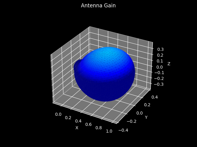
class Dipole(mode=AntennaMode.DUPLEX, pose=None)

Bases: Generic[APT], Antenna[APT]

Model of vertically polarized half-wavelength dipole antenna.

Dipole Antenna Characteristics

The assumed characteristic is

\[\begin{split}F_\mathrm{V}(\phi, \theta) &= \frac{ \cos( \frac{\pi}{2} \cos(\theta)) }{ \sin(\theta) } \\ F_\mathrm{H}(\phi, \theta) &= 0\end{split}\]

Parameters:

• mode (AntennaMode, optional) – Antenna’s mode of operation. By default, a full duplex antenna is assumed.

• pose (Transformation, optional) – The antenna’s position and orientation with respect to its array.

copy()

Create a deep copy of the antenna.

Return type:

Dipole

Returns:

A deep copy of the antenna.

local_characteristics(azimuth, elevation)

Generate a single sample of the antenna’s characteristics.

The polarization is characterized by the angle-dependant field vector

\[\begin{split}\mathbf{F}(\phi, \theta) = \begin{pmatrix} F_{\mathrm{H}}(\phi, \theta) \\ F_{\mathrm{V}}(\phi, \theta) \\ \end{pmatrix}\end{split}\]

denoting the horizontal and vertical field components. The directional antenna gain can be computed from the polarization vector magnitude

\[\begin{split}A(\phi, \theta) &= \lVert \mathbf{F}(\phi, \theta) \rVert \\ &= \sqrt{ F_{\mathrm{H}}(\phi, \theta)^2 + F_{\mathrm{V}}(\phi, \theta)^2 }\end{split}\]

Parameters:

• azimuth (float) – Considered horizontal wave angle in radians \(\phi\).

• elevation (float) – Considered vertical wave angle in radians \(\theta\).

Return type:

ndarray

Returns:

Two dimensional numpy array denoting the horizontal and vertical ploarization components of the antenna response vector.

yaml_tag: Optional[str] = 'DipoleAntenna'

YAML serialization tag

class IdealAntenna(mode=AntennaMode.DUPLEX, pose=None)

Bases: Generic[APT], Antenna[APT], Serializable

Theoretic model of an ideal antenna.

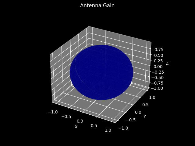
Ideal Antenna Characteristics

The assumed characteristic is

\[\begin{split}\mathbf{F}(\phi, \theta) = \begin{pmatrix} \sqrt{2} \\ \sqrt{2} \\ \end{pmatrix}\end{split}\]

resulting in unit gain in every direction.

Parameters:

• mode (AntennaMode, optional) – Antenna’s mode of operation. By default, a full duplex antenna is assumed.

• pose (Transformation, optional) – The antenna’s position and orientation with respect to its array.

copy()

Create a deep copy of the antenna.

Return type:

IdealAntenna

Returns:

A deep copy of the antenna.

local_characteristics(azimuth, elevation)

Generate a single sample of the antenna’s characteristics.

The polarization is characterized by the angle-dependant field vector

\[\begin{split}\mathbf{F}(\phi, \theta) = \begin{pmatrix} F_{\mathrm{H}}(\phi, \theta) \\ F_{\mathrm{V}}(\phi, \theta) \\ \end{pmatrix}\end{split}\]

denoting the horizontal and vertical field components. The directional antenna gain can be computed from the polarization vector magnitude

\[\begin{split}A(\phi, \theta) &= \lVert \mathbf{F}(\phi, \theta) \rVert \\ &= \sqrt{ F_{\mathrm{H}}(\phi, \theta)^2 + F_{\mathrm{V}}(\phi, \theta)^2 }\end{split}\]

Parameters:

• azimuth (float) – Considered horizontal wave angle in radians \(\phi\).

• elevation (float) – Considered vertical wave angle in radians \(\theta\).

Return type:

ndarray

Returns:

Two dimensional numpy array denoting the horizontal and vertical ploarization components of the antenna response vector.

yaml_tag: Optional[str] = 'IdealAntenna'

YAML serialization tag

class LinearAntenna(mode=AntennaMode.DUPLEX, slant=0.0, pose=None)

Bases: Generic[APT], Antenna[APT], Serializable

Model of a linearly polarized ideal antenna.

The assumed characteristic is

\[\begin{split}\mathbf{F}(\theta, \phi, \zeta) = \begin{pmatrix} \cos (\zeta) \\ \sin (\zeta) \\ \end{pmatrix}\end{split}\]

with \(zeta = 0\) resulting in vertical polarization and \(zeta = \pi / 2\) resulting in horizontal polarization.

Initialize a new linear antenna.

Parameters:

• mode (AntennaMode, optional) – Antenna’s mode of operation. By default, a full duplex antenna is assumed.

• mode – Antenna’s mode of operation. By default, a full duplex antenna is assumed.

• slant (float) – Slant of the antenna in radians.

• pose (Transformation, optional) – Pose of the antenna.

copy()

Create a deep copy of the antenna.

Return type:

LinearAntenna

Returns:

A deep copy of the antenna.

local_characteristics(azimuth, zenith)

Generate a single sample of the antenna’s characteristics.

The polarization is characterized by the angle-dependant field vector

\[\begin{split}\mathbf{F}(\phi, \theta) = \begin{pmatrix} F_{\mathrm{H}}(\phi, \theta) \\ F_{\mathrm{V}}(\phi, \theta) \\ \end{pmatrix}\end{split}\]

denoting the horizontal and vertical field components. The directional antenna gain can be computed from the polarization vector magnitude

\[\begin{split}A(\phi, \theta) &= \lVert \mathbf{F}(\phi, \theta) \rVert \\ &= \sqrt{ F_{\mathrm{H}}(\phi, \theta)^2 + F_{\mathrm{V}}(\phi, \theta)^2 }\end{split}\]

Parameters:

• azimuth (float) – Considered horizontal wave angle in radians \(\phi\).

• elevation (float) – Considered vertical wave angle in radians \(\theta\).

Return type:

ndarray

Returns:

Two dimensional numpy array denoting the horizontal and vertical ploarization components of the antenna response vector.

property slant: float

Slant of the antenna in radians.

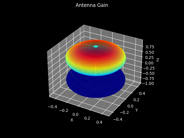
class PatchAntenna(mode=AntennaMode.DUPLEX, pose=None)

Bases: Generic[APT], Antenna[APT], Serializable

Realistic model of a vertically polarized patch antenna.

Patch Antenna Characteristics

Refer to Jaeckel et al.[1] for further information.

Parameters:

• mode (AntennaMode, optional) – Antenna’s mode of operation. By default, a full duplex antenna is assumed.

• pose (Transformation, optional) – The antenna’s position and orientation with respect to its array.

copy()

Create a deep copy of the antenna.

Return type:

PatchAntenna

Returns:

A deep copy of the antenna.

local_characteristics(azimuth, elevation)

Generate a single sample of the antenna’s characteristics.

The polarization is characterized by the angle-dependant field vector

\[\begin{split}\mathbf{F}(\phi, \theta) = \begin{pmatrix} F_{\mathrm{H}}(\phi, \theta) \\ F_{\mathrm{V}}(\phi, \theta) \\ \end{pmatrix}\end{split}\]

denoting the horizontal and vertical field components. The directional antenna gain can be computed from the polarization vector magnitude

\[\begin{split}A(\phi, \theta) &= \lVert \mathbf{F}(\phi, \theta) \rVert \\ &= \sqrt{ F_{\mathrm{H}}(\phi, \theta)^2 + F_{\mathrm{V}}(\phi, \theta)^2 }\end{split}\]

Parameters:

• azimuth (float) – Considered horizontal wave angle in radians \(\phi\).

• elevation (float) – Considered vertical wave angle in radians \(\theta\).

Return type:

ndarray

Returns:

Two dimensional numpy array denoting the horizontal and vertical ploarization components of the antenna response vector.

yaml_tag: Optional[str] = 'PatchAntenna'

YAML serialization tag

class UniformArray(element, spacing, dimensions, pose=None)

Bases: Generic[APT, AT], AntennaArray[APT, AT], Serializable

Model of a Uniform Antenna Array.

Parameters:

• element (Type[AT] | AT | APT) – The element uniformly repeated across the array. If an antenna is passed instead of a port, a new port is automatically created.

• spacing (float) – Spacing between the elements in m.

• dimensions (Sequence[int]) – The number of elements in x-, y-, and z-dimension.

• pose (Tranformation, optional) – The anntena array’s transformation with respect to its device.

property antennas: List[AT]

All individual antenna elements within this array.

property base_port: APT

Base port repeated across the array topology.

property dimensions: Tuple[int, ...]

Number of antennas in x-, y-, and z-dimension.

Returns: Number of antennas in each direction.

property num_antennas: int

Number of antenna elements within this array.

property ports: Sequence[APT]

Sequence of all antenna ports within this array.

property spacing: float

Spacing between the antenna elements.

Returns:

Spacing in m.

Return type:

float

Raises:

ValueError – If spacing is less or equal to zero.

[1]

Stephan Jaeckel, Kai Borner, Lars Thiele, and Volker Jungnickel. A geometric polarization rotation model for the 3-d spatial channel model. IEEE Transactions on Antennas and Propagation, 60(12):5966–5977, 2012. doi:10.1109/TAP.2012.2214017.